WOMBAT! (for estimating CO₂ sources and sinks)

In 2015, together with Noel Cressie, I started looking at the problem of estimating sources and sinks of greenhouse gases such as methane and carbon dioxide using ideas from spatial and spatio-temporal statistics. We quickly realised that this is an extremely difficult and inter-disciplinary problem, which requires a team with expertise in high-performance computing, atmospheric chemistry, and statistics.

In the early years (2015/2016) Noel and I did some in-roads in developing multivariate statistical models for use in regional flux inversion, drawing on expertise from the atmospheric chemists at my former host institution, the University of Bristol (Matt Rigby, Anita Ganesan, and Ann Stavert), and published two papers on this, one in the journal Chemometrics and Intelligent Laboratory Systems and another in the journal Spatial Statistics. Following this, we started looking into global inversions from OCO-2 (a NASA satellite) data. Progress was slow initially, but in 2018 Noel and I were successful in acquiring Australian Research Council grant money with which we managed to recruit Michael Bertolacci, a research fellow with the perfect skill set and inter-disciplinary mindset, and this is when the project really took off. Two years later, we are participants in the next global OCO-2 model intercomparison project (MIP) and contributors to a COP26 Global Carbon Stocktake product. Our final flux inversion system is called WOMBAT, which is short for the WOllongong Methodology for Bayesian Assimilation of Trace Gases, and a manuscript describing it has now been accepted for publication with Geophys ical Model Development. Other essential contributors to WOMBAT development include Jenny Fisher and Yi Cao, and we have had help from many others too as we acknowledge in the paper.

Wombat in Cradle Mountain, Australia. Photo by Meg Jerrard.

The Model

At the core of WOMBAT is a Bayesian hierarchical model (BHM) which establishes a flux process model, (i.e., a model for the sources and sinks), a mole-fraction process model (i.e., a model for the spatio-temporal evolving atmospheric constituent), and a data model, which characterises the relationship between the mole-fraction field and the data that are ultimately used to infer the fluxes. A summary of the BHM is given below:

The underlying Bayesian hierarchical model used in WOMBAT.

Each of these models is very simple to write down mathematically, but involves quite a lot of work to implement correctly. First, note from the above schematic that the flux process model involves a set of flux basis functions: these need to be extracted/constructed from several published inventories. We use inventories that describe ocean fluxes, fires, biospheric fluxes, and several others, so that the basis functions have spatio-temporal patterns that are reasonably similar to what could be expected from the underlying flux.

Second, the mole-fraction process model involves running a chemical-transport (numerical) model. The chemical-transport model we used is GEOS-Chem, which is a global 3-D model that can simulate the transport and chemical reactions of gases when supplied with meteorological data as input. Running chemical-transport models is nerve-wracking as they have a lot of settings and input parameters: a small mistake can result in a lot of wasted computing time or, even worse, go undetected. The chemical-transport model is needed to see what the effect of the CO₂ fluxes is on the atmospheric mole fraction, which is ultimately what the instruments are measuring. Of course we are relying on the model and the met fields we use as being ”good enough,” but we also account for some of the errors they introduce through v₂ in the above schematic. In WOMBAT we acknowledge that these errors may be correlated in space and time, and employ a simple spatio-temporal covariance model to represent the correlation. This correlation has the effect of considerably increasing our uncertainty on the estimated fluxes (i.e., ignoring the correlation can lead to over-confident estimates).

Finally, the data themselves are highly heterogeneous. In this paper we focus on OCO-2 data, which are available to us as column-retrievals (i.e., the average dry air mole fraction of carbon dioxide in the atmosphere in a sometimes vertical, often skewed, column from the satellite to the surface of Earth). These data are actually the product of a retrieval algorithm which is itself an inversion algorithm, and are biased and have errors of their own. We account for all of this in the data model, which contains many parameters that need to be estimated. We use Markov chain Monte Carlo (Metropolis-within-Gibbs) to estimate all the parameters in our model.

Findings

So, what do we find out? First, from the methodological perspective we find that if biases are indeed present in the data, and that if correlations in the errors are not taken into account when they are really there, that flux estimates can be badly affected. Several inversion systems currently in place do not take these into account, largely because data are already largely de-biased prior to being used in an inversion, but primarily because taking into account correlations is computationally difficult. We also show that estimating biases while doing the inversion is possible, and that offline de-biasing can be complemented in this way. Second, from a science point of view, we show that our flux estimates are largely in line with those from other inversion systems and that (unsurprisingly!) carbon dioxide injection in the atmosphere is very high, with humans to blame for this. Below, we show our estimates of total carbon dioxide surface flux, split by land and ocean, excluding fossil fuel emissions, using data from a specific satellite mode (Land Glint [LG]). We also show the flux estimates from the first OCO-2 model intercomparison project (MIP), which largely agree with our estimates. Note how Earth absorbs about 4 PgC (i.e., petagrams of Carbon) per year on average. Unfortunately, humans are emitting on the order of 10 PgC per year of CO₂ into the atmosphere. This big discrepancy in flux (approximately 6 PgC per year) means that carbon dioxide levels in the atmosphere will only keep on increasing, and have a deleterious effects on the climate we have learnt to live with. With WOMBAT, as with most flux inversion systems, we can also zoom in to see where and when most carbon dioxide is being emitted or absorbed. This will become a main focus of ours moving forward when preparing our submission to the COP26 Global Carbon Stocktake product.

Annual (left column) and monthly (right column) fluxes for the globe (first row), land (second row), and ocean (third row). Summaries of flux estimates from the model intercomparison project (MIP) and the flux estimate from WOMBAT are shown, split into the prior and LG inversions.

We are currently implementing several exciting upgrades to WOMBAT. For more information about the project, please do not hesitate to get in touch!

Multi-Scale Process Modelling and Distributed Computation for Spatial Data

I recently published a paper, joint with Jonathan Rougier, on modelling, and computing with, multi-scale spatial processes (click here for the arXiv version). A multi-scale spatial process is, simply put, a superposition of processes with differing spatial scales, where each component process has its own ‘spectral signature,’ or ‘frequency bandwidth.’ The first process captures coarse scales. The second process captures finer scales, and so on.

Global map of sea-surface temperature anomaly produced from approx. 1,000,000 data points, using a spatial process model with two scales. Left panel: Prediction (posterior mean). Right panel: Uncertainty (posterior standard error).

Computing with multi-scale spatial processes is not easy. A straightforward way to proceed would be to introduce some notion of independence at the finer scales, by first tiling up the process and then separately computing with variables and parameters associated with these tiles. While this approach brings with it an ease for modelling nonstationarity, it does not yield a realistic, global, model; indeed the process at the finer scale is deemed to be discontinuous at the boundaries of the tiles. The main aim of this work was to come up with a computational strategy to avoid the independence assumption, while allowing one to model nonstationarity at the finer scales.

The strategy we converged on is the following:

1. Model the process as a sum of independent Gaussian Markov random fields (GMRFs) to take advantage of sparse linear algebraic libraries when making inference.
2. Associate each GMRF with a spatial scale, and use informative prior distributions to ‘separate’ the scales associated with each GMRF.
3. Model the first (coarse) scale GMRF as stationary, and subsequent GMRFs as nonstationary, with increasing degrees of nonstationarity (faster fluctuating length scales, etc.) with decreasing scale.
4. Define each GMRF over a tessellation of the domain of interest, where finer tessellations are associated with GMRFs with finer scales.
5. Use the conditional independence and distribution properties of GMRFs (exploiting graph colouring and collapsed distributions) to generate a Markov chain associated with the process that mixes well and converges quickly to the target (posterior) distribution.

A colouring of the spatial domain in the global sea-surface temperature application. Each colour contains process variables at the fine scale that are sampled concurrently within a Gibbs sampling framework.

This paper took many years in the making (about 6 years), partially because it was always a project ‘on the side,’ but also because we were not happy with early iterations of the model. In the first model iteration we only assumed one scale, and simply took advantage of the computational benefits of GMRFs via graph colouring to make inference computationally efficient, but the novelty associated with this single-scale model was questionable: both graph colouring and nonstationary GMRFs are not new, although to the best of my knowledge they have not been treated together.

In the second model iteration we introduced multiple scales, but assumed spatial block-independence at these finer scales. This created posterior standard errors and predictions that were very unrealistic, with sharp discontinuities at the boundaries. I still have an early image of the meshing strategy we adopted, which I show below.

Our second model iteration of a two-scale process on the sphere used a coarse mesh (with vertices at the blue dots, just about visible) superimposed on separately-constructed fine meshes (with vertices at the yellow dots). Overlap of the fine meshes was introduced to reduce the effect of boundary conditions.

In the third model iteration we considered global models for the finer scales as well, and used a graph colouring scheme together with a small approximation to the conditional distribution (eq. 11 in the paper) to make inference on the finer scale component of the processes. This worked well, but GMRF variables close to the boundaries of the tiles, created for the purpose of graph colouring, did not mix well. Furthermore, there was no smoothness constraint on the spatial variances and length scales, which is problematic. I found an image of this early attempt, where I show serious issues with the prediction standard error at the boundaries of the tiles used for graph colouring, together with unrealistic heterogeneity..

Prediction standard errors using our third model iteration, which did not have any smoothness constraints on the spatially-varying variances and length scales, and did not allow for good mixing of the Markov chain at the boundaries of the tiles used for graph colouring. Note how the poor mixing manifests itself in poor estimates of the prediction standard error at the tile boundaries.

In the fourth model iteration we used basis functions to model the variances and length scales of the GMRF at the finer scale, and introduced a series of rotating tiling/colouring schemes. The latter modification solved the mixing issues we had at the boundaries. This final model ‘felt right;’ it worked well, both from a representational point of view, and a computational point of view. The posterior prediction and prediction standard error maps using this fourth iteration are shown at the beginning of this blog post, where we effectively model (and not just predict) globally the sea-surface temperature at a 30 x 30 km resolution (we can predict at much higher resolutions if we want to).

Three tilings of our domain used in our Gibbs sampler to alleviate the problem of poor mixing at tile boundaries.

All in all this project was very rewarding, and I believe it has provided a demonstrable advance in spatial modelling and computation. The results compellingly show an improvement over other state-of-the-art methods for spatial prediction. The only real downside of this approach is the effort required to implement it: it requires one to construct informative prior distributions, manually tessellate the domain, and run a Gibbs sampler for several days for a problem with approximately 1,000,000 data points! Options are currently being explored to automate and speed up the modelling and fitting procedures, but, at the time of writing, there does not seem to be an easy way forward.

Reproducible code for this project is available here.

Convolution Neural Networks for Statistical Spatio-Temporal Forecasting

An article that I co-authored with Chris Wikle has just been published in a Special Issue edited by Alan Gelfand with the journal Spatial Statistics. An arXiv version is here while the reproducible code can be found here. The methodology in this paper is one which I find very exciting — it essentially takes a framework that has recently appeared in Machine Learning and sets it firmly within a hierarchical statistical modelling framework.

The idea behind it all is relatively simple. Spatio-temporal phenomena are generally governed by diffusions and advections that are constantly changing in time and in space. Modelling these spatio-temporally varying dynamics is hard, estimating them is even harder! Recently, de Bézenac et al. published this very insightful paper showing how, using ideas taken from solving the optical flow problem, one can train a convolution neural network that takes as input an image sequence exhibiting the spatio-temporal dynamics, and spouts out a map showing the spatially-varying advection parameters. The idea is simple: Let the CNN see what happened in the past few time instants and it will tell you in which direction things are flowing, and the strength at which they are flowing! They use a convolution neural network (CNN) to make this happen.

Their code was written in PyTorch, but since R has got an awesome TensorFlow API I decided to make my own code using their architecture and see if it works. I honestly am not sure how ‘deconvolution’ works in a CNN (which is part of their architecture), so what I did was implement a version of their CNN where I just go into a low-dimensional space and stay there (I then use basis functions to go back to my original domain). Without going into details, the architecture we ended up with looks like this:

Figure 1: CNN which takes a sequence of images as inputs and outputs parameters that can reconstruct spatially-varying diffusions and advections.

The performance was impressive right from the start… even on a few simple image sequences of spheres moving around a domain we could estimate dynamics really well.

But de Bézenac’s framework has a small problem — it only works for complete images which are perfectly observed. What happens if some of the pixels are missing or the images are noisy? Well, this is where hierarchical statistical models really come in useful. What we did was recast the CNN as a (high-order) state-space model, and run an ensemble Kalman filter using it as my ‘process model.’ The outcome is a framework which allows you to do extremely fast inference of spatio-temporal dynamic systems with little to no parameter estimation! (Disclaimer: when using a CNN that is already trained!)

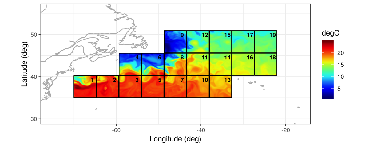
To show the flexibility of this methodology we trained the network on about 80,000 sequences of (complete) images of sea-surface temperature from a publicly available data set (the same data set used by de Bézenac et al., see the image at the top of this page and the video here), and then used it to predict the advection parameters of a Gaussian kernel moving in space (which we just simulated ourselves). The result is impressive — even though none of the training images resemble a Gaussian kernel moving in space, the CNN can tell us where and in which direction ‘stuff’ is moving. The CNN has essentially learnt to understand basic physics from images.

Figure 2: Output flow direction and intensity from the fitted CNN (arrows) in response to a Gaussian radial basis function shifting in time (contours), with decreasing transparency used to denote the function at times t − 2, t − 1 and t, respectively.

All of this gets a bit more crazy — we used the CNN in combination with an ensemble Kalman filter to nowcast rainfall. Remember that we trained this CNN on sea-surface temperatures! The nowcasts were better in terms of both mean-squared prediction error and continuous-ranked probability score (CRPS) than anything we could throw at it (uncertainties appear to be very well-calibrated with this model). To add icing on the cake, it gave us the nowcast in a split second… Have a look at the article for more details.

Deep Compositional Spatial Models

This week I arXived a paper I wrote with Tin Lok James Ng (University of Wollongong), Quan Vu (University of Wollongong), and Maurizio Filippone (Eurecom), titled Deep Compositional Spatial Models. As the name implies, the paper describes a spatial model that is inspired by deep learning, specifically, deep Gaussian processes.

To understand why these deep spatial models might be interesting objects, we need a brief run through history. Sampson & Guttorp, back in 1992, published a paper in JASA promoting the idea of warping a spatial domain and modelling simple (stationary) processes on this warped domain. On this warped domain all process realisations appear to be simple and regular; when plotted on the unwarped domain though, they can appear rather complex. Spatial warping is thus a long standing method to model spatial processes that exhibit complicated behaviour (i.e., processes that are highly nonstationary).

Enter deep neural nets, which are designed to model complex warpings such as the one we envisage. The basic idea in our paper is to warp space using neural net architectures, and then proceed with modelling the process on this warped space. This has been done before in various guises, but what is new here is that we model elementary bijective warpings used to generate the global warping through composition as random (non-Gaussian) processes. Bijectivity is important, as it guarantees that the warping does not fold. As with other deep process models, we also take advantage of the technologies used in deep learning, such as TensorFlow.

The random bijective warping is achieved by modelling each warping layer as a trans-Gaussian process (since Gaussian maps cannot guarantee bijectivity). Therefore, each layer is itself a nonlinear transformation of a Gaussian process. While this may appear to complicate things, in fact, the sample paths of these bijective maps are very constrained and, somewhat paradoxically, I found that the deep (non-Gaussian) warping is very easy to fit since the solution space has practically been decimated to only contain those maps that are bijective.

So what we end up with is a model that has random warpings, that does not result in ‘space folding,’ and that is easy and very quick to fit using GPUs. To give you an idea, our 1D examples required only a couple of seconds for fitting and prediction, while our 2D examples required a couple of minutes. Compare this to the DGPRFF where we needed a day of careful optimisation to get a good fit, and MCMC (elliptical slice sampling) on a deep Gaussian process (ala Schmidt & O’Hagan) that needed nearly a week to ‘converge.’ The model is sufficiently complex, yet also sufficiently parsimonious, a win-win situation for spatial problems (or other very low-dimensional problems) where pathologies due to over-warping are likely.

From a spatial statistician’s point of view, what is attractive is that there is very little effort needed to model the stretches, anisotropies, etc., that worry us so much. The ability to capture the ‘directions of flow’ is remarkable. See the following pictures for example; in each one, the top-left panel shows the true warping; the top-right panel shows the recovered warping from simulated data (that is only identifiable up to a rigid transformation); and the bottom three panels show the truth, the prediction, and the prediction standard error, respectively. The prediction standard errors clearly follow the process ‘contours’ — this is desirable but not something you’d get using standard kriging or Gaussian process regression.

• 

• 

Each of the following two images compares the deep spatial model predictions (middle row), to those from a standard Gaussian process (bottom) when fitting MODIS image data (top-right, subsampled from the complete data, top-left). The first one is particularly interesting since the image is taken over Antarctica. Since luminescence over Antarctica is practically constant in this image, the warping collapses Antarctica to nearly a single point, so that uncertainty over Antarctica is practically nill. On the other hand the predictions and prediction errors capture the major directions of variation in the images. The difference of these predictions to those from a standard Gaussian process regression is striking.

• 

• 

All in all this was a very exciting project with some excellent colleagues who assisted in the writing and the simulation experiments. Maurizio, in addition, provided some valuable hands-on advice for getting stochastic variational Bayes to work, which was a crucial component of this work.

The idea for this project came from a very inspiring workshop  I had attended at Imperial College, over 5 years ago, specifically from a talk by James Hensman on variational encoders. I remember walking back with James to the train station and discussing with him the models with a view on how they could be used in spatial statistics. I’m very glad to see they work so well in practice, so thank you James for the inspiration!

Geostatistics in the fast lane using R-TensorFlow and GPUs

On 28th May 2019 at 6pm I will be giving a talk at the Annual Joint SSA Canberra and R-Ladies Event in Canberra on the use of GPUs for solving simple problems in geostatistics. I’m going to do it ‘workshop-style’ and hopefully give the attendees some (brief) hands-on experience with TensorFlow. Here are the details:

Date: Tuesday 28 May 

5.20pm Refreshments in Foyer, Ground level, Building 145 (Where is the Hanna Neumann (MSI) building?).

6.00pm Presentation in Room 1.33, Building 145  

In my talk I will briefly discuss spatial modelling and Gaussian process regression, and then describe TensorFlow and RStudio’s API to it. At the end of the talk I will show how one can implement maximum likelihood estimation in a geostatistical context using TensorFlow, and illustrate the speed improvement when using a GPU. The vignette I will be going through can be found here. Attendees are invited to bring their own laptop to run some simple commands I mention in the talk and the code in the vignette.

 

Workshop: Spatio-Temporal Statistics with R (Sydney, 29-30 April 2019)

The Course

Noel Cressie and myself are offering a workshop at the UOW Sydney Business School, on 29/30 April. This 1.5-day workshop is based on our recent book that is freely available for download from https://spacetimewithr.org. It considers a systematic approach to analysing spatio-temporal data, with a particular emphasis on hierarchical (empirical and Bayesian) statistical modelling. The workshop, which is endorsed as an activity of the Environmental Statistics Section of the Statistical Society of Australia (SSA) , will cover the following topics in spatio-temporal statistics.

• Key concepts of hierarchical modelling; overview of requisite background in spatial statistics.
• Data wrangling with spatio-temporal data.
• Spatio-temporal data classes in R.
• Visualisation of spatio-temporal data using lattices and grammar of graphics.
  EDA for spatio-temporal data (including visualisation and empirical dimension-reduction) in R.
• Standard statistical models for spatio-temporal data.
• Covariance functions and spatio-temporal kriging in practice.
• Rank-reduced spatio-temporal modelling approaches.
• Dynamic spatio-temporal modelling.

For more information and registration details visit niasra.uow.edu.au

Research Fellow (Postdoc) position at the University of Wollongong, Australia

The Centre for Environmental Informatics (CEI) in the School of Mathematics and Applied Statistics conducts world-leading research in high-level statistical methodology and statistical computing and their application to the environmental sciences.

The postdoctoral Research Fellow will work in the centre with Prof Noel Cressie, Dr Andrew Zammit Mangion, and environmental scientists on the recently awarded Australian Research Council (ARC) grant, “Bayesian inversion and computation applied to atmospheric flux fields.” The project aims to make use of unprecedented sources of measurements, from remote sensing and in situ data, to estimate the sources and sinks of greenhouse gases. This will be solved in the context of Bayesian spatio-temporal inversion and big-data computational strategies.

The requirements for this position are:

• PhD degree in Statistics/Statistical Science
• Strong programming skills in R, Python, or MATLAB
• Demonstrated expertise in Bayesian methods and computation
• Ability to work effectively in a multi-disciplinary team on the main UOW campus in Wollongong

Closing Date: 01/04/2019, 11:59:00 PM (AEDT)
Salary Details: Level B: $98,019 – $113,353 + 17% superannuation

 

For more details and to apply please visit here.

 

Our book is now published and available online!

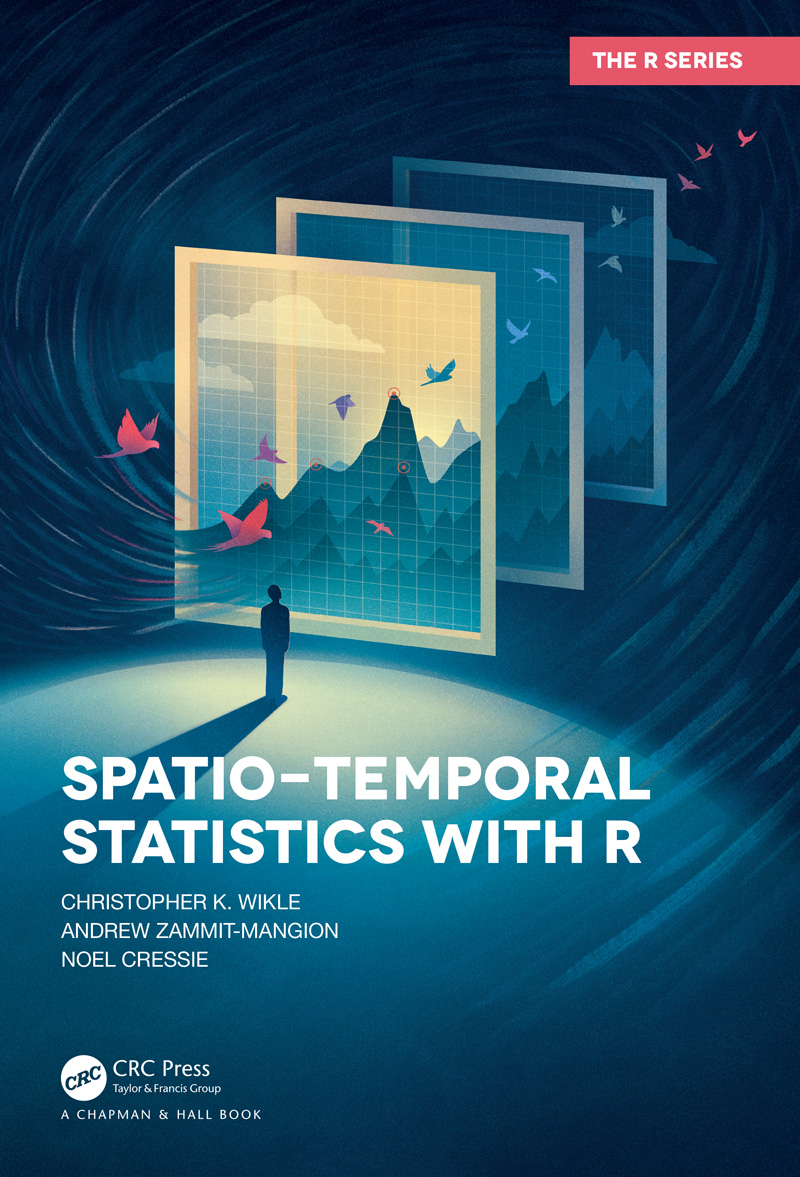
Our new book Spatio-Temporal Statistics with R has now been published with Chapman & Hall/CRC. It was a great few years writing this book with Chris Wikle and Noel Cressie, and I’m overjoyed to see the finished product. The book can be downloaded for free here. A hard-cover edition of the book can be purchased from Chapman & Hall/CRC here (Discount code: ASA18).

Summary

The world is becoming increasingly complex, with larger quantities of data available to be analyzed. It so happens that much of these “big data” that are available are spatio-temporal in nature, meaning that they can be indexed by their spatial locations and time stamps.

Spatio-Temporal Statistics with R provides an accessible introduction to statistical analysis of spatio-temporal data, with hands-on applications of the statistical methods using R Labs found at the end of each chapter. The book:

• Gives a step-by-step approach to analyzing spatio-temporal data, starting with visualization, then statistical modelling, with an emphasis on hierarchical statistical models and basis function expansions, and finishing with model evaluation
• Provides a gradual entry to the methodological aspects of spatio-temporal statistics
• Provides broad coverage of using R as well as “R Tips” throughout.
• Features detailed examples and applications in end-of-chapter Labs
• Features “Technical Notes” throughout to provide additional technical detail where relevant
• Supplemented by a website featuring the associated R package, data, reviews, errata, a discussion forum, and more

The book fills a void in the literature and available software, providing a bridge for students and researchers alike who wish to learn the basics of spatio-temporal statistics. It is written in an informal style and functions as a down-to-earth introduction to the subject. Any reader familiar with calculus-based probability and statistics, and who is comfortable with basic matrix-algebra representations of statistical models, would find this book easy to follow. The goal is to give as many people as possible the tools and confidence to analyze spatio-temporal data.

 

 

R coding tips for spatio-temporal analyses

If you are into spatio-temporal modelling and its applications, you probably are also spending a good deal of your time coding in R and seeing ways in which you can enhance your code for better performance. As we start to work routinely with “big data,” i.e. data sets on the order of several Gb and even Tb in raw form, there is no room for complacency. We need to have good well-structured, modular, well-tested and reusable code. When dealing with data on these scales it is very easy to get frustrated when testing out a prototype, or for mistakes to go unnoticed and “lost in transmission.” Here I provide some random tips which can help reduce development time and the number of logical errors in code and package design of these sort of programs.

1. Use md5 for caching

Md5 is a hashing algorithm which produces a “unique” (i.e. unique for practical purposes) number based on the data being digested. This is particularly useful when you want to execute a set of operations on a chunk of code which will take a long time.

The trivial way of by-passing this is by executing the code, then saving the data, for example using save in R, commenting out the code and adding a load after the commented code. This is bad practice for one very good reason, if variables or data on which we are executing change, this will go unnoticed and we can end up with a program which is mixing old results with new results during development. The other option, to run the sequence of instructions every time we test the code is equally prohibitive.

This is where md5 comes in. We digest all the input variables and data before the sequence of code and produce a hash number. We then check a designated folder (I use a /cache folder in the project directory) for a filename which is the same as the hash number. If it is there we load it, otherwise we execute the commands and save into the cache using the md5 as filename at the end. This has the advantage that this block of code will only be run IF any of the input variables/data change. Working in an environment where people change the data or “apply new corrections” all the time? No problem, this md5 wrapper around the code will do all the work for you.

In R this wrapper will look something like this:

md5 <- digest(file=args$path,algo="md5")
if(check_md5(md5)) {
    cat("Found existing MD5 for data. Loading...", sep = "\n")
    load(file = file.path("./cache",paste(md5,".rda",sep="")))
} else {
.
.
.
  save(.Object,file=file.path("./cache",paste(md5,".rda",sep="")))
}

where check_md5 is a small function which checks the folder for the required file.

2. Do not code, design

It is very tempting in applications such as these to start coding without thought for the big picture, or package development. Unfortunately everything we do is pretty much useless if it cannot be ported into an entirely different setting with minimal user effort. If we want our work to be useful to the wider audience, we should code for re-usability. This will lengthen development time considerably, but the end result will be something useful which can help others.

I believe (and I should stress that this is just personal opinion), that the key to producing reusable code which can be ported across applications, is the use of an object-oriented paradigm. This is not because imperative programming cannot be used to produce re-usable code, rather that object-oriented programming is naturally designed to let you do this neatly.

The potential advantages of using OO code are numerous. For example, in spatio-temporal applications we usually make use of classes of basis functions which have different properties but which all serve the same purpose. In this case I can  define a class of basis functions, which can include the finite element basis (used in Lindgren et al, 2011), the bisquare functions (Cressie et al.), EOFs (Wikle et al.), spherical harmonics and so on. All these classes will share a common interface with methods such as “interpolate” or “plot” and “find_Gram_matrix”, all common functions in spatio-temporal modelling. I can then formulate spatial and spatio-temporal models in the same way, irrespective of the basis I’m using.

For the actual modelling we can then create another class called “gmrf” with the required properties (precision and mean) and associate this with a set of basis functions. The vector autoregressive model would be a subclass of the “gmrf” class and builds a GMRF based on parameters I construct it with. The spatial CAR model would be another sub-class and so on. In this way we can construct multivariate spatio-temporal modelling problems with different basis, a mix of spatial/temporal basis functions etc. with little effort. The  FRK package I have recently released has code built on this premise

3. Use low-level languages sparingly buy wisely

There is no greater satisfaction than writing something in C++ and linking it through Rcpp, or using RcppArmadillo, and having to blink at the speed of your new code. We encounter many operations that can benefit from low-level code in spatio-temporal analyses (e.g., computing Euclidean distances). Unfortunately, though, you still need to know how to code in C++. Speaking for myself, I feel I have lost touch with low-level programming languages, and I’m not as confident as I once used to be. Even with the goldmines of Rcpp and RcppArmadillo at my fingertips I still find myself spending time recalling how to incorporate C++ in R, and how to code in C++. Nowadays what I do is I make sure the whole program is written and tested in R, then find the bottlenecks and see whether they can be speeded up using low-level code. I still keep the Rfunctions; I then use the C++ implementations and the Rimplementations in test functions (see next point).

4. Test, test, test…

Automatic testing has come of age in R through the testthat package. Coding individual units and not proceeding until they pass a range of tests (in a strict bottom-up approach) is tedious, but you will reap the benefits later. In automatic testing, the tests can be re-run after every change you make, to ensure nothing has “broken.” You can also design the tests in such a way so that not only small functions are tested, but even full-scale analysis, where you know roughly what the outcome can be. For example if coding up simple kriging, you can have tests that verify that your matrix calculations for computing prediction variances are correct, or you can do kriging on simulated data with a fixed seed (so that the result is reproducible), and throw an error if the predictions are off in some sense. Both these type of tests can be used to warn you of problems that arise from a change that you effect in the code. Testing is particularly useful with continuous-integration systems such as Travis CI, and test coverage reports can be generated to show you how much of your code is being tested.

5. Think carefully about function interfaces

While code within functions can change without any user being the wiser, the function interface cannot. It is therefore time well spent thinking what the function will be used for, now, and in the future. For example, if you are fitting a model using the EM algorithm, but want to allow the possibility of other estimation methods being implemented in the future, include a “method” argument which can be used to indicate the fitting method in the future. Think also about the ordering of the arguments, and put the most important arguments that are likely to last the test of time first in your function definition.

6. Use useful variable names

In an application I’m currently working on, I’m having to deal with differing units, lengths in m and km, masses in kg, T, MT and GT, densities in kg per km2m and so on. My first attempt of keeping track was to comment next to the variable name what the variable constant refers to. However, a variable name such as rho_kg_km2m or area_km2 immediately reflects the quantity we are talking about.

Judicious use of variable names goes beyond indicating the units. Frequently, the symbols used in the code do not match up with that published in an accompanying paper on which the code is based. This can be extremely confusing to reviewers and to end users. Although there is a big barrier to changing symbol names used in code, this should be of high priority when there is an accompanying manual or publication.

Notes from DSSV 2017 (Conference)

The inaugural conference on Data Science, Statistics and Visualisation (DSSV2017) was an interesting change from other conferences. The audience was mixed, with a good proportion (roughly 50%) coming from industry. Many sessions reminded me of the Meetups that occur in Sydney, the balance between talks containing math and other talks remaining at a high level was appealing.

In this conference I talked about the medal plot, a graphic for visualising uncertainty in space-time fields that was developed by Jonty Rougier and myself during my stay in Bristol. The medal plot can be used to see the effect of considering spatial correlations in your model, and the effect of your prior judgement on your posterior uncertainties. More details are given in our paper here.

The conference opened with an interesting talk by Trevor Hastie who gave a run-through of subset selection methods before introducing a new one: Relaxed LASSO. Interesting points, some of which we are aware of already:

• In Trevor’s experience, forward subset selection is (in practice) as good as best subset selection, but of course orders of magnitude faster. Forward selection works with n < p unlike, of course, backward selection.
• An exhaustive search for best subset selection can be easily carried out on up to 35 covariates using the leaps package in R.
• Recently Bertsimas, King, and Mazumder cracked the best-subset selection curse of dimensionality using mixed-integer programming and the GUROBI solver (which can be used in R). However is best subset selection always the best? No, it tends to overfit the data.
• LASSO can be seen as a “convex relaxation” of the best-subset selection problem (which has an L0 penalty term instead of an L1, and is hence admits a non-convex cost function).
• In GLMNET, LASSO is implemented using pairwise coordinate descent and computes the optimal solution over a fine grid of the regularisation parameter lambda.
• Trevor spent some time talking about the connections between Least-Angle Regression, LASSO, and forward subset selection which was interesting.
• In Relaxed LASSO (which was new to me) one uses LASSO to obtain the non-zero terms. Then one computes a linear combination of the LASSO estimates and the OLS estimates of those non-zero terms. Note that this is different from elastic net, in which the cost function contains both an L1 and an L2 penalty, but is similar in spirit. Trevor claimed that this reduces the shrinkage bias in vanilla LASSO methods.
• Trevor showed the results of an extensive simulation study containing experiments with different SNRs and covariate intra-correlations. Interestingly, the best subset and forward subset selection methods only outperformed the LASSO methods at high SNRs. The relaxed LASSO consistently outperformed LASSO.

Another talk I found very interesting was that by Andre Martins on constructing sparse probability distributions by replacing the ubiquitous softmax function with a sparsemax function. More details are given in his paper here. The problem is formulated as an optimisation problem, where one is projecting the weights onto the probability simplex. While I guess this part is not new, Andre constructed a loss function inspired by that of the softmax to obtain simple optimisation algorithms.

David Banks talked about emulation of agent-based models (ABMs), something which I am personally sceptical about since ABMs are useful because they are chaotic in nature, a feature emulators would struggle to capture. Yet, when I enquired about this, David said he and his student had considerable success in emulation and that the discrepancy term is able to capture the “unpredictable component” in ABMs fairly well so I will keep an open mind on this one!

On the last day we had several interesting talks. Mario Figueiredo talked about the OSCAR loss function which deals with correlated variables in a different way than LASSO. While LASSO will assign all the weight to one of the correlated variables, OSCAR will assign equal weight to the correlated variables. There is an interesting connection between the “shrinking to exactly zero” of the LASSO and the “shrinking to exactly the same weight for correlated variables” of the OSCAR criterion. Mario extended this to an OWL criterion which generalises the OSCAR criterion (but I’m not sure in what way!).

Peter Rousseeuw talked about detecting cell-wise outliers (as opposed to row-wise outliers) in data. He showed some impressive figures obtained using his package cellWise. The Technometrics paper describing the technique is here. I do have an issue with calling outliers and anomalies the same, something which every speaker asserted in this conference. In my opinion, an outlier is a property of the data, while an anomaly is a property of the process. That is, an outlier is something we would like to filter out, while an anomaly is something we would like to keep, model, and even predict!

After Peter, Google (with three speakers) gave a talk on market attribution models that involved using non-stationary Markov models to simulate user behaviour. Finally, Daniel Keim gave a very impressive talk on visual analytics. He took the audience through a graphical journey involving Twitter feeds for disaster detection, IP monitoring for attack detection, and the analysis of soccer team strategies from millisecond data of players’ positions on the field. All this was after lambasting statisticians somewhat for solving “small” problems using only “selective” data (but which we do “very well”).

I of course do not agree with Daniel; we do what we do not because we are scared of dealing with “very” big data, but because it is not always necessary to work with all the data one could possibly collect, to solve big problems. I think Daniel focuses on some important fields which indeed do require a lot of data (and which is hence technologically very challenging), but I disagree that that is  always”the real world”. Further, like in visual analytics, we also use process chains (starting from data collection, to data pre-processing, to feature selection, to modelling, to inference, to visualisation) much like what is needed in the truly big-data cases he described.

One point which concerned me what that there was no mention of uncertainty. This is not a problem when raw data is displayed, but when an inference is conveyed, decision-making on a point prediction without a notion of risk can be dangerous.

One of the graphics Daniel showed which I never tire of seeing was Anscombe’s quartet:

Source: https://en.wikipedia.org/wiki/Anscombe%27s_quartet

All the four data sets shown above have the same marginal means, the same correlation coefficient, and the same best linear fit. Daniel used this to emphasise the importance of visualisation. An extreme case of this is shown in this lovely video below by Justin Matejka; this is an excellent resource for STAT101!